The Causality-Driven Company
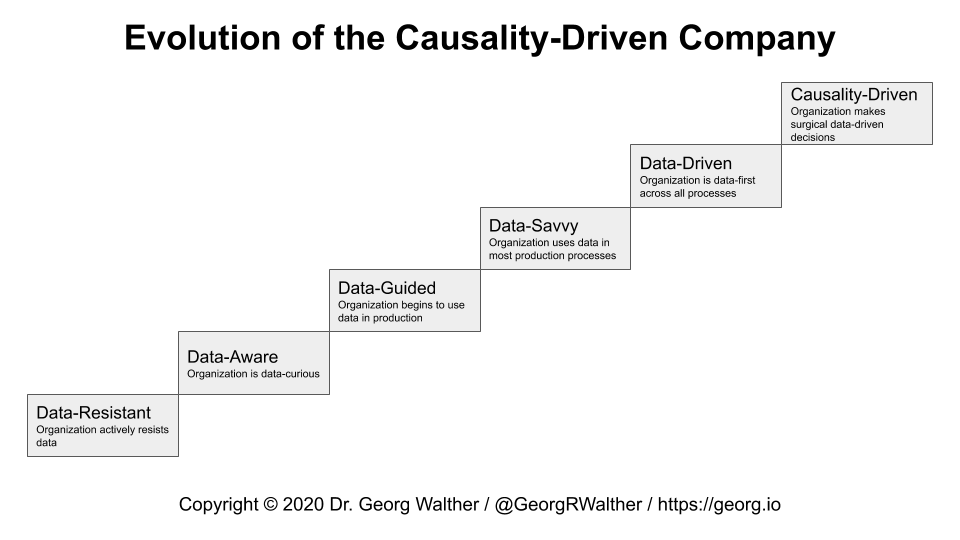
Increasingly, enterprises embrace decision-making based on data, thus becoming data-driven companies. However, decisions based purely on data can lead to mistakes and may waste resources. Combining causal models with data promises to fix these issues. In this article I explain why the causality-driven company is the sensible step up from the data-driven company.
- The data-driven company
- Machine learning applications for the data-driven company
- Smart manufacturing
- The missing piece: causality
- Becoming a causality-driven company
The data-driven company
Much has been written on data being the new oil and enterprises needing to embrace big data and machine learning to benefit in three important ways:
- Utilizing existing resources more efficiently thus reducing cost,
- Increasing success rates thus increasing revenue, and
- Developing entirely new revenue streams thus diversifying their business.
Enterprises are said to be data-driven once their entire organization is data-first, meaning:
- Both their core processes (e.g. production lines) and supporting processes (e.g. recruiting) are quantifiable through transparent metrics, and
- All business units have a data mindset, i.e. are driven by testable hypotheses, and have the technological means for it.
Machine learning applications for the data-driven company
There a numerous applications of big data and machine learning in industry and the enterprise. Common applications include:
- Predictive maintenance,
- Demand forecasting,
- Optimal pricing,
- Intelligent routing,
- Data-driven customer support (e.g. chatbots), amd
- Churn prediction.
Another key application in industry is smart manufacturing which promises to decrease cost and increase both production line output and quality.
Smart manufacturing
Product quality prediction
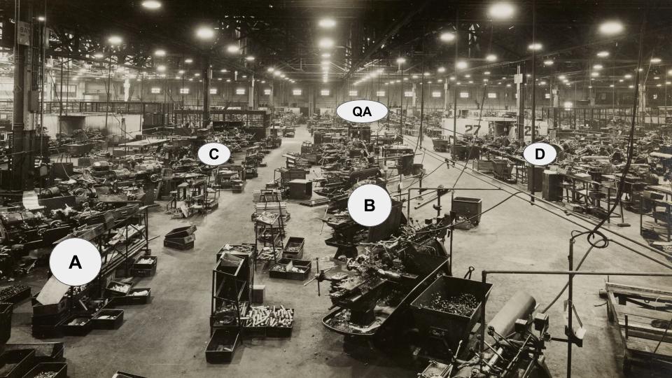
Consider our production line, pictured above in Figure 1, which consists of a number of workstations that the different parts of our product need to pass through before being assembled into our final product.
The various workstations can be described by parameters, e.g. how much pressure or force is applied, how fast a tool is spinning, or categories such as the type of drill used.
Our fictional production line above has four production parameters spread across its workstations: , , , and .
At the far end of our production line the quality of our assembled product is quantified in the quality assurance gateway (). Here, either an employee or a machine visually inspects or physically tests manufactured items to verify their quality before they are shipped to customers.
Since our company is data-driven we collect data on every item coming off our production line. Such a data set may look as follows:
| Product ID | Timestamp | A | B | C | D | QA |
|---|---|---|---|---|---|---|
| … | … | … | … | … | … | … |
| 123 | 2020-05-10 14:35:00 | 1.2 | 102.1 | ZZ | YY | 0.98 |
| 456 | 2020-05-10 16:20:00 | 1.1 | 104.3 | ZZ | XX | 0.96 |
| 789 | 2020-05-11 06:04:00 | 1.3 | 100.6 | ZX | YY | 0.83 |
| 012 | 2020-05-11 10:45:00 | 1.1 | 101.3 | ZX | YZ | 0.92 |
| … | … | … | … | … | … | … |
Parameters and of our production line are numerical features while parameters and are categorical features. Our quality measurement is a numerical target variable which takes values between 0 and 1 with the latter representing the highest possible product quality.
Provided that we collect enough production line data, machine learning offers a rich toolbox for predicting the expected score or whether our score will lie above a certain threshold. The former application is called regression (predict value) while the latter is called classification (predict if is greater than a threshold).
To implement these applications there are numerous established machine learning models, some of which are:
- Linear and polynomial regression,
- (Deep) neural networks / deep learning,
- Classification and regression trees (CART),
- Ensemble methods such as random forests and gradient tree boosting,
- Logistic regression,
- Support vector machines,
- Gaussian processes, and
- Naive Bayes.
These machine learning models allow us to learn the potentially complex relationship between our production line parameters (, , , and ) and resultant product quality ().
These are also the same machine learning models used routinely to implement the other aforementioned industry applications such as demand forecasting or churn prediction.
So training a machine learning model on our production line data we get something like this:
.
Where our model predicts the quality of our final product based on the parameters of our production line.
Using our prediction model
Imagine we manage to train a highly accurate machine learning model on our production line data - what do we do with it?
Sure, if measuring the quality of our product () is prohibitively expensive we could cut cost by using our model to determine the quality score for items coming off our production line.
We could also try and adapt our model so that it provides accurate quality score predictions early in the production cycle for a given item - thus allowing us to cancel work on substandard items before they consume resources unnecessarily.
But really, what we are most likely interested in is:
How should we tweak individual production parameters to increase product quality?
Issue with our prediction model
Unfortunately, our machine learning model does not hold the answer to our core question: Out of the box it will not help us optimize individual production parameters to improve our quality score .
Let’s see why that is.
We can write our machine learning model as a function:
where is our model that predicts the quality score for items manufactured with production parameters , , , and .
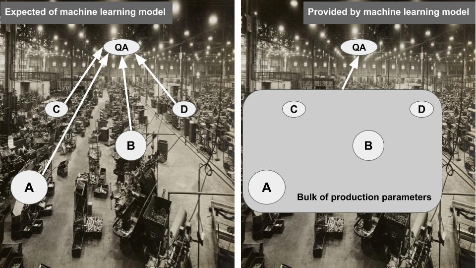
The issue with this model is that it learns the relationship between quality score and production parameters “in bulk” - or in other words the conditional distribution of jointly on production parameters , , , and .
The only sensible operation we can carry out with this model is asking all production line workers for their presently (or planned) production parameter values, inputting them into our model, and informing our colleagues in production of the quality score we expect to achieve with their configuration.
Of course, a far more desirable operation would be to take the presently used production parameters, e.g.
tweak a single parameter, e.g. increase parameter by 10%, and compute the newly expected quality score
If the newly predicted turns out greater than the presently achieved or predicted quality score we would go back to the production floor and ask our colleague manning the workstation to increase their parameter by 10%.
Unfortunately, this operation of tweaking and optimizing individual input variables (production parameters) is not supported by our machine learning model.
In essence, our model learns the bulk relationship between the entire set of production parameters and quality score, and not the individual impact of each production parameter on the quality score - as illustrated in the following sketch:
This problem pertains to most machine learning models independent of the specific problem tackled.
How do we modify our approach so that we can estimate the impact of individual production parameter modifications and help our colleagues on the production floor make optimal, surgical changes to their manufacturing process?
One major piece to closing this gap is causality.
The missing piece: causality
Variables and parameters are often interconnected
To disentangle their individual contributions, we first need to account for how our production parameters influence one another and the quality score.
To understand the connections between our production parameters and the quality score, we pop down to the production floor and chat with our colleagues manning the individual workstations. From them we learn:
- When the stiffness of the raw material (A) increases then downstream workers increase the pressure applied on the item (B),
- Depending on the stiffness of the raw material (A) the type of downstream drill (C) is chosen,
- The worker choosing the type of drill (C) also informs the worker moulding our item under pressure (B) since they need to balance bore friction and metal stiffness,
- The worker applying a specific type of finish (D) to our product is not affected by the choices of their co-workers.
Armed with these insights from our production floor we draw up the following causal model - showing the connections among our production parameters and the quality score of our product:
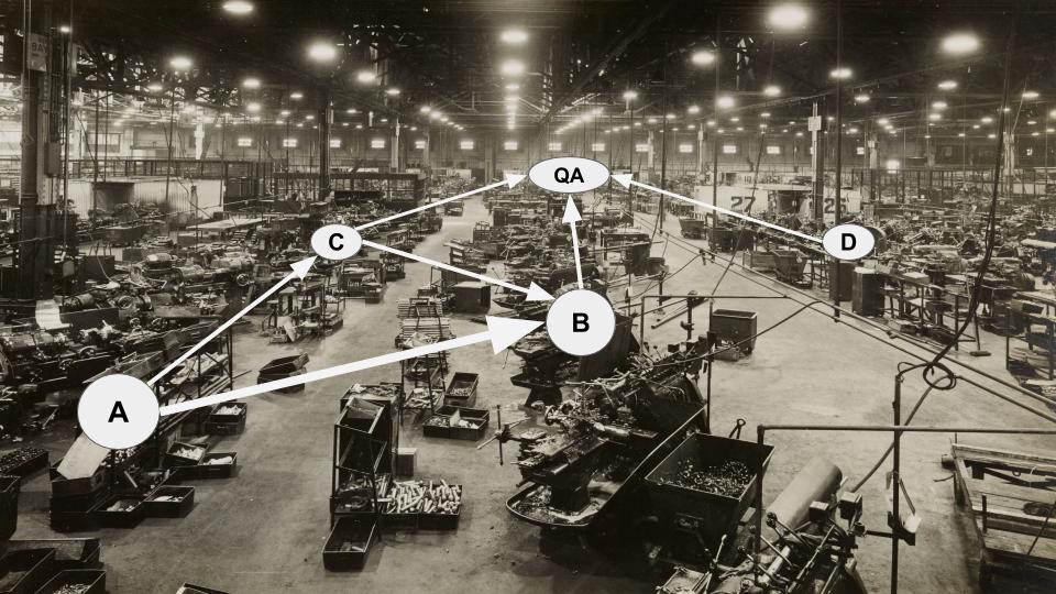
A simplistic, and perhaps crude, way of interpreting the arrows between parameters , , and is to imagine these arrows were unidirectional mechanical springs. If I pull on parameter by changing it somehow, I also move around parameters and - however pulling on does not affect as that spring is unidirectional.
Interconnected variables are hard to disentangle
To reiterate, our main use for a machine learning model that predicts the quality score of manufactured items is to support our colleagues on the production floor in optimizing individual production parameters to maximize our overall output quality.
Our causal model (Figure 3) makes it apparent that our model should be more complex than previously thought. The connections in our causal model indicate that we should write our model as
where both and are functions of
.
In short: In addition to teaching our machine learning model the relationship between our four production parameters and the quality score, we also need to teach our model the various relationships between our production parameters before we can use our model to optimize individual workstations.
To learn all these relationships we need a lot of data and variation in production parameters that show how the parameters influence one another. We may be inclined to go down to the manufacturing floor and start experimenting at random with our production parameters generating enough data to learn both the interconnections between the production parameters (, ) and their individual impact on our quality score .
However, each manufactured item with substandard quality due to a randomly selected combination of production parameters means money lost for our company.
This approach, called randomized experiment or randomized controlled trial, is oftentimes undesirable or simply infeasible:
- In the case of our production line (and smart manufacturing in general), randomly assigning production parameters to measure their individual impact would be both very time consuming and prohibitively expensive - imagine all the low-quality items made and discarded,
- In e-commerce, for smart pricing, it is in fact prohibited by law to price the same item differently for different customers in the same market,
- In customer care it would be counterproductive to treat some customers poorly just to see how their purchase behavior and brand loyalty are affected,
- In predictive maintenance it would be questionable or prohibited not to perform best practice maintenance steps on individual items to see how they deteriorate differently, and
- In online marketing it is ofentimes prohibitively complex or infeasible, due to data protection legislation, to cleanly understand the effect (uplift) of isolated marketing parameters on individual users.
Hence, we cannot rely on randomized experiments to understand how to optimally help our production floor colleagues.
So what we are left with is continue doing what we do on the production floor, and use the production data generated under normal operating conditions (observational data) to estimate the impact of each production parameter individually on our quality score.
To achieve this we need to rely on both our causal model (Figure 3) and a toolset from the field of causal inference called do-calculus.
Causal inference toolset: Do-calculus
The components we have gathered so far are:
- A causal model of our production floor (Figure 3), and
- Lots of observational data of production parameter settings and measured resultant quality score .
Let us go through a thought experiment illustrated in the image below (Figure 4): How would the expected quality score change if our colleague in workstation chose their production parameter independently of their colleagues in workstations and ?
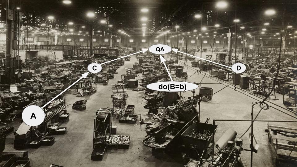
This is what the notation in Figure 4 relates to: describes a theoretical scenario where production parameter is assigned to hold value - instead of a scenario where parameter is observed to equal value .
Note the seemingly subtle but important difference: If we go back to our observational data generated under normal operating conditions then observing implies something about production parameters and since, according to our causal model (Figure 3), these are causally connected! However, forcing (or intervening on) parameter by setting it to value breaks that causal link between the workstations - and this is what the notation signifies.
In essence would mean asking our colleague in workstation to stop listening to their colleagues in workstations and .
Since doing so in reality on the production floor would incur high cost due to lost production we simulate the intervention ! using the observational data we collect under normal operating conditions anyway.
To simulate we apply a set of algebraic rules, called do-calculus, to our causal model from Figure 3 and draw on our regular observational data from the production floor.
In technical terms, do-calculus allows us to turn theoretical interventional distributions into regular conditional distributions that we can compute using our observational data.
With this toolset we can finally estimate the individual effect of tweaking production parameter on quality score thus allowing us to optimize surgically our manufacturing output.
Becoming a causality-driven company
I hope I managed to convince you of the important difference between recording lots of data and being able to optimize individual steps of your business operations based on your data.
The former is limited to prediction: Your organization can predict future outcomes if all internal processes continue to be operated as usual. This is the essence of the data-driven company.
The latter adds explanation to prediction: Your organization can explain how outcomes and future outcomes come about. And once you can explain how your processes lead to outcomes you can start optimizing individual components of your processes and organization. This enables you to analyze what would happen if you changed “the way you have always done things” - thus elevating you to a causality-driven company.
How can you start using causal inference and tools such as do-calculus to optimize your business? And how do you eventually become a causality-driven company?
A roadmap of this kind, a causality strategy if you will, would certainly be an interesting subject for another blog article.
Until then, I would start by becoming a data-driven company first:
- Set up data collection across all key operations of your business,
- Start working on machine learning prototypes for predicting key business metrics based on your collected data, and
- Start asking yourself: Once I can predict my business metrics with machine learning, what specific changes should I make to my business to optimize these metrics?
Once you get to the point of wanting to make surgical decisions based on your machine learning model, causality and causal inference will start playing key roles.
