Multiclass classification applied to a stream of documents in Python
In this article we implement multiclass classification on an online stream of documents implemented in Python.


I recently joined a Kaggle competition on multilabel text classification and have learned a ton from basic code that one of the competitors shared in the forums.
The code of the genereous competitor does logistic regression classification for multiple classes with stochastic gradient ascent. It is further well-suited for online learning as it uses the hashing trick to one-hot encode boolean, string, and categorial features.
To better understand these methods and tricks I here apply some of them to a multilabel problem I chose mostly for the easy access to a constant stream of training data:
All recent changes on Wikipedia are tracked on this special page where we can see a number of interesting features such as the length of the change, the contributor's username, the title of the changed article, and the contributor's comment for a given change.
Using the Wikipedia API to look at this stream of changes we can also see how contributors classify their changes as bot, minor, and new. Multiple label assignments are possible, so that one contribution may be classified as both bot and new.
Here I will listen to this stream of changes, extract four features (length of change, comment string, username, and article title), and train three logistic regression classifiers (one for each class) to predict the likelihood of a change belonging to each one of them. The training is done with the stochastic gradient ascent method.
One caveat: I am a complete novice when it comes to most of this stuff so please take everything that follows with a grain of salt - on the same note I would be forever grateful for any feedback especially of the critical kind so that I can learn and improve.
%matplotlib inline
import matplotlib
from matplotlib import pyplot as pt
import requests
import json
from math import log, exp, sqrt
from datetime import datetime, timedelta
import itertools
from collections import defaultdict
The API that Wikipedia offer to listen to the stream of recent changes is described here.
URL = ('http://en.wikipedia.org/w/api.php?format=json&action=query&list=recentchanges&rcprop=parsedcomment'
      '%7Ctimestamp%7Ctitle%7Cflags%7Cids%7Csizes%7Cflags%7Cuser&rclimit=100')
The logistic regression classifier requires us to compute the dot product between a feature vector $\mathbf{x}$ and a weight vector $\mathbf{w}$.
$$\mathbf{w}^\text{T} \mathbf{x} = w_0 x_0 + w_1 x_1 + w_2 x_2 + \ldots + w_N x_N.$$
As by convention, the bias of the model is encoded with feature $x_0 = 1$ for all observations - the only thing that will change about the $w_0 x_0$-term is weight $w_0$ upon training. The length of the article change is tracked with numerical feature $x_1$ which equals the number of character changes (hence $x_1$ is either positive or negative for text addition and removal respectively).
As in the Kaggle code that our code is mostly based upon, string features are one-hot encoded using the hashing trick:
The string features extracted for each observed article change are username, a parse of the comment, and the title of article. Since this is an online learning problem there is no way of knowing how many unique usernames, comment strings, and article titles are going to be observed.
With the hashing trick we decide ab initio that D_sparse-many unique values across these three features are sufficient to care about:
Our one-hot encoded feature space has dimension D_sparse and can be represented as a D_sparse-dimensional vector filled
with 0's and 1's (feature not present / present respectively).
The hash in hashing trick comes from the fact that we use a hash function to convert strings to integers.
Suppose now that we chose D_sparse = 3 and our hash function produces
hash("georg") = 0, hash("georgwalther") = 2, and hash("walther") = 3 for three observed usernames.
For username georg we get feature vector $[1, 0, 0]$ and for username georgwalther we get $[0, 0, 1]$.
The hash function maps username walther outside our 3-dimensional feature space and to close this loop we not only
use the hash function but also the modulus (which defines an equivalence relation?):
hash("georg") % D_sparse = 0, hash("georgwalther") % D_sparse = 2, and hash("walther") % D_sparse = 0
This illustrates one downside of using the hashing trick since we will now map usernames georg and walther to the same feature vector $[1, 0, 0]$.
We are therefore best adviced to choose a big D_sparse to avoid mapping different feature values to the same one-hot-encoded feature - but probably not too big to preserve memory.
For each article change observation we only map three string features into this D_sparse-dimensional one-hot-encoded feature space - out of D_sparse-many vector elements there will only ever be three ones among (D_sparse-3) zeros (if we do not map to the same vector index multiple times).
We will therefore use sparse encoding for these feature vectors (hence the sparse in D_sparse).
We will also normalize the length of change on the fly using an online algorithm for mean and variance estimation.
D = 2  # number of non-sparse features
D_sparse = 2**18  # number of sparsely-encoded features
def get_length_statistics(length, n, mean, M2):
    """ https://en.wikipedia.org/wiki/Algorithms_for_calculating_variance#Incremental_algorithm """
    n += 1
    delta = length-mean
    mean += float(delta)/n
    M2 += delta*(length - mean)

    if n < 2:
        return mean, 0., M2

    variance = float(M2)/(n - 1)
    std = sqrt(variance)
    return mean, std, M2

def get_data():
    X = [1., 0.]  # bias term, length of edit
    X_sparse = [0, 0, 0]  # hash of comment, hash of username, hash of title
    Y = [0, 0, 0]  # bot, minor, new

    length_n = 0
    length_mean = 0.
    length_M2 = 0.

    while True:
        r = requests.get(URL)
        r_json = json.loads(r.text)['query']['recentchanges']
        for el in r_json:
            length = abs(el['newlen'] - el['oldlen'])
            length_n += 1
            length_mean, length_std, length_M2 = get_length_statistics(length, length_n, length_mean, length_M2)
            X[1] = (length - length_mean)/length_std if length_std > 0. else length

            X_sparse[0] = abs(hash('comment_' + el['parsedcomment'])) % D_sparse
            X_sparse[1] = abs(hash('username_' + el['user'])) % D_sparse
            X_sparse[2] = abs(hash('title_' + el['title'])) % D_sparse

            Y[0] = 0 if el.get('bot') is None else 1
            Y[1] = 0 if el.get('minor') is None else 1
            Y[2] = 0 if el.get('new') is None else 1

            yield Y, X, X_sparse
def predict(w, w_sparse, x, x_sparse):
    """ P(y = 1 | (x, x_sparse), (w, w_sparse)) """
    wTx = 0.
    for i, val in enumerate(x):
        wTx += w[i] * val

    for i in x_sparse:
        wTx += w_sparse[i]  # *1 if i in x_sparse

    try:
        wTx = min(max(wTx, -100.), 100.)
        res = 1./(1. + exp(-wTx))
    except OverflowError:
        print wTx
        raise

    return res
def update(alpha, w, w_sparse, x, x_sparse, p, y):
    for i, val in enumerate(x):
        w[i] += (y - p) * alpha * val
    for i in x_sparse:
        w_sparse[i] += (y - p) * alpha  # * feature[i] but feature[i] == 1 if i in x
K = 3
w = [[0.] * D for k in range(K)]
w_sparse = [[0.] * D_sparse for k in range(K)]
predictions = [0.] * K
alpha = .1
time0 = datetime.now()
training_time = timedelta(minutes=10)

ctr = 0
for y, x, x_sparse in get_data():
    for k in range(K):
        p = predict(w[k], w_sparse[k], x, x_sparse)
        predictions[k] = float(p)
        update(alpha, w[k], w_sparse[k], x, x_sparse, p, y[k])

    ctr += 1

    # if ctr % 10000 == 0:
        # print 'samples seen', ctr
        # print 'sample', y
        # print 'predicted', predictions
        # print ''

    if (datetime.now() - time0) > training_time:
        break
ctr
As we can see, we crunched through 106,401 article changes during our ten-minute online training.
It would be fairly hard to understand the link between the D_sparse-dimensional one-hot-encoded feature space and
the observed / predicted classes.
However we can still look at the influence that the length of the article change has on our classification problem
print w[0]
print w[1]
print w[2]
Here we can see that the weight of the length of change for class 0 (bot) is -1.12, for class 1 (minor) is -0.97, and for class 2 (new) is 2.11.
Intuitively this makes sense since many added characters (big positive change) should make classification as a minor change less likely and classification as a new article more likely: For an observed positive character count change $C$, $2.11 C$ will place us further to the right, and $-0.97 C$ further to the left along the $x$-axis of the sigmoid function:
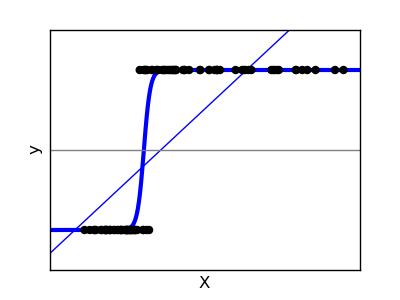 (from http://gaelvaroquaux.github.io/scikit-learn-tutorial/supervised_learning.html#classification)
Further below we will see that the vast majority of bot changes are classified as minor changes hence we would expect to see correlation between the weights of this feature for these two classes.
To further evaluate our three classifiers, we observe another 10,000 Wikipedia changes and construct a confusion matrix.
no_test = 10000
test_ctr = 0

classes = {c: c_i for c_i, c in enumerate(list(itertools.product([0, 1], repeat=3)))}
confusion_matrix = [[0 for j in range(len(classes))] for i in range(len(classes))]

predicted = [0, 0, 0]
for y, x, x_sparse in get_data():
    for k in range(K):
        p = predict(w[k], w_sparse[k], x, x_sparse)
        predicted[k] = 1 if p > .5 else 0
    i = classes[tuple(y)]
    j = classes[tuple(predicted)]
    confusion_matrix[i][j] += 1
    test_ctr +=1

    if test_ctr >= no_test:
        break
matplotlib.rcParams['font.size'] = 15
fig = pt.figure(figsize=(11, 11))
pt.clf()
ax = fig.add_subplot(111)
ax.set_aspect(1)
res = ax.imshow(confusion_matrix, cmap=pt.cm.jet, interpolation='nearest')
cb = fig.colorbar(res)
labels = [{v: k for k, v in classes.iteritems()}[i] for i in range(len(classes))]
pt.xticks(range(len(classes)), labels)
pt.yticks(range(len(classes)), labels)
pt.show()
The confusion matrix shows actual classes along the vertical and predicted classes along the horizontal axis.
The vast majority of observed classes are $(0, 0, 0)$ and our classifiers get most of these right except that some are misclassified as $(0, 0, 1)$ and $(0, 1, 0)$.
All observed bot-related changes (classes starting with a $1$) are $(1, 1, 0)$ (i.e. minor bot-effected changes) and our classifiers get all of those right.